Workshop 1 Introduction to R
If you haven’t already installed R, it is available here. Then, download R Studio.
Welcome to the first R for Psychological Science workshop! This workshop is intended for people who want to learn R, but don’t know much about it or have recently started using it.
Here’s what we are going to learn in this workshop to get you started in R:
How does the R interface work? How do I use it to write code?
What’s the logic behind how R works?
How can I get my data into R?
1.1 Getting started: How to use RStudio and R Markdowns
Welcome to using R! I recognize that for many of us this is our first time seeing R–or any coding language for that matter–and it might feel a bit overwhelming. Don’t worry, you’ll get there! In this workshop, I will try to make your introduction to using R as clear and helpful as possible. Even still, it might be a lot to take in the first time. Feel free to revisit or review as you need–It’s very normal to have to give material for learning R a few passes at first to start and internalize it.
Alright, let’s jump in!
For this workshop, we are going to use two really helpful tools that help us use R effectively (and more easily):
- R Studio
- R Markdown
Almost everyone that uses R uses R Studio–this is essentially the default way of interacting with R. In the next section, we’ll dive into how to understand the R Studio interface and feel comfortable using it. For your reference, R Markdown is also very popular, but sometimes people also use other similar tools like R Scripts or R Notebooks, so you will probably see each of these types used in practice. I’ll make an argument below for why I like using R Markdown.
1.1.1 Explaining R Studio
R Studio is the program that we open up and write R code in. But, as you have seen at this point, you actually have to download R and R Studio separately. How, then, are R and RStudio different? RStudio is an interface that overlays the program R and is more user-friendly. It is the way that you interact with R. You can think of R as an engine and R Studio as the body of the car, which let’s you use that engine to get places. R, on it’s own, is literally just a blank box on your screen (what we call a console) where you can type and run code. In contrast, here’s what the default RStudio interface looks like on Windows:
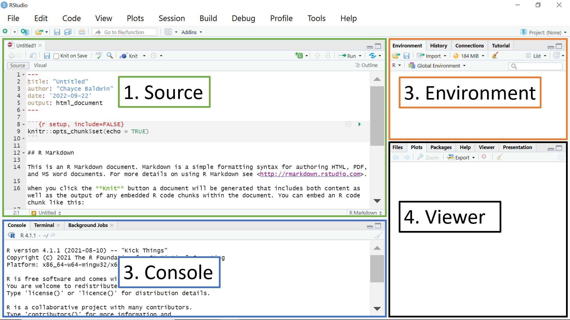
RStudio has the same Console pane as R. Additionally, it has 3 other panes: as an Environment pane where you can see all the variables and datasets you’ve saved in your R session, a Viewer pane where you can access your files, view your plots, access your packages, and get help, and a Source pane where you can create R Markdown documents (or R scripts or Notebooks).
How to create a new doc and to save stuff How to change the theme
1.1.2 Let’s use R Studio for R Markdowns
So, what is an R Markdown document? This is the main kind of document that I use in RStudio, and it’s one big advantage of RStudio over the base R console. As I’ve mentioned, if you’re interested in what else you can do in R Studio, the other common types of documents in R Studio are the R script and R notebook.
R Markdown allows you to create a file with a mix of R code and regular text, which is useful if you want to have explanations of your code alongside the code itself, write up results of your analyses, better organize your code, or even write up answers to a homework assignment in your stats class. This document, for example, is an R Markdown document. It is also useful because you can export your R Markdown file to an html page or a PDF, which comes in handy when you want to share your code or a report of your analyses to someone who doesn’t have R. For example, this R Markdown file has been exported into an html page so you can see it online.
If you’re interested in learning more about the functionality of R Markdown, you can visit this webpage. Also, out of the goodness of their hearts, the team at RStudio literally made a cheat sheet for R Markdowns. Check it out. Not only that, they have made cheat sheets for a lot of other things as well…We’ll get into those later.
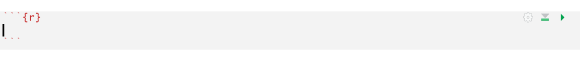
R Markdowns are organized as chunks where you write code, with spaces in between that you can write text. A chunk is designated by starting with three ticks and {r} and ending with three ticks (```), and is shown as a grey box (in the default RStudio theme). In the space between chunks, you can write text to help you organize your analyses, write out results, or anything else! In this R Markdown for this workshop, all of the text I have written is in between code chunks. Here’s what a chunk will look like:
A new chunk can be created by pressing COMMAND + OPTION + I on Mac, or CONTROL + ALT + I on PC.
You can run lines of code from your chunk by placing the cursor anywhere in the line of code, and pressing COMMAND + ENTER on Mac, or CONTROL + ENTER on PC. If you want to run a whole chunk of code, you can press COMMAND + ALT + C on Mac, or ALT + CONTROL + ALT + C on PC, or you can press the little green arrow in the top right corner of the chunk (see the picture above).
1.2 Part I: What you need to know to use R
At its least useful, you can treat R like a calculator for basic computations. Just type some mathematical expression into your code chunk, and the result will be displayed in the console (the bottom left pane of R Studio) as well as just below your chunk.
## [1] 3## [1] 6.5## [1] 64## [1] 25Beyond that, there are two fundamental ideas that will provide a framework for everything we do in R:
- Using objects
- Using functions
1.2.1 Using objects
One of the big picture, fundamental things about R: Everything in R is an object. Anytime we want to use, manipulate, analyze, or save data, we assign it to an object, and those objects are what we use for everything in R. When we assign values to an object, we can also call this a variable–so you can interchangeably use or think about this as objects or variables.
1.2.1.1 What is object assignment?
You can think of object assignment as just meaning that we take a value or group of values and putting them in a box with a given name, so that we can use them later. This essentially describes the basic process that underlies everything we do in R: we take all of the numbers we have, all the functions we have (we’ll talk more about those later), and anything else and we put them in these “boxes” called objects. Then we interact those boxes with each other to manipulate, analyze, or present or data in the ways we want.
Say, for example, we want to take the number 4 and assign it to x. Then, one way of thinking about it is “putting 4 in a box called x”. Another way of saying this is x gets the value 4.There are two (almost) equivalent ways to do this:
In both cases, x will represent 4 for all lines of code below these here.
## [1] 4## [1] 4It is important not to confuse variable assignment with a statement about equality. In your head, you should say set x to 4 or x gets 4, but not x is equal to 4. Don’t worry now about the subtle differences between the two assignment styles. Although using = is more consistent with the norm in other programming languages, I prefer <- as it makes the action that is being performed more obvious. Whichever you choose, it’s best to be consistent throughout your code.
One other thing to notice: see how on the line after assigning 4 to the object x we just have x all by itself? When you run a line of code that is just an object name, without doing anything else to it, R will tell us what is in the object, printing the contents in the console.
1.2.1.2 Naming objects
Since we use these “boxes” called objects for just about everything, it’s worth spending a minute to think about how to name them.
It’s fine to use variable names like x for simple math examples like the ones above. But, I’ll give you a little tip that will save you time, confusion, and stress in the future: when writing code to perform analysis, use descriptive names. Code where things are named subject_id, condition, and rt will be a bit more verbose than if you had used x, y, and z, but it will also make much more sense when you read it again 4 months later as you write up the paper.
With that said, there are a few rules for variable names. You can use any alphanumeric character (i.e., a-z and 0-9), although the first character must be a letter. You can’t use spaces, because the computer doesn’t know that you’re trying to write a phrase and interprets that as two (or more) separate terms. When you want something like a phrase, the _ and . characters can be used to connect words or numbers (this can be a bit confusing as . is usually meaningful in programming languages, but not in R). For example:
#using letters
se <- 22

#using letters and numbers
se1 <- 22

#using _
self_efficacy1 <- 22

#using .
self.efficacy1 <- 22
In R, you will see _ and . used all of the time for names of things–this is normal (and maybe even the only?) way of making names that are more than one word or term. Throughout this workshop, you’ll see we use them all the time for naming objects and they are used all the time in function names, too. This is how we do R speak :)
OK, great–those are some basics about variable assignment.
Here’s a simple example that novice coders often find confusing. Walk yourself through the code and make sure you understand what operations lead to the final value given when we print (i.e., show the value of) a:
## [1] 20That’s right, an object will only contain its most recent assignment. Even though a was originally given the value 10, it was then reassigned the value of b, which had the value of 20.
1.2.1.3 Types of data in objects
So far we’ve only been dealing with numbers, but there are other data types as well. Imagine education research using college admission essays, or marketing research which has data on what different brands a consumer purchased from, or social psychological research with data on whether or not people who had committed crimes were repeat offenders. Each of these examples uses different type of data that R recognizes as unique and can be used in different ways.
In the first instance, college admission essays would be text data, which we call “character” or “string” data. Character/string values are assigned with quotation marks:
## [1] "average"Here, even though we used letters for one object and digits for the other, R recognizes both objects as character values. Using quotation marks makes all input into character strings.
Do you see how rsc_phone changes when we don’t use quotation marks?
## [1] 2018675309Without quotation marks, R recognizes the digits as a number that can be operated on–it can be added, subtracted, etc.
Now consider the data of whether or not people who have committed a crime are repeat offenders. One way to think about this data is thinking of each person as having a value answering the question, “Is this person a repeat offender?”, where they get a “yes” or a “no”. In R, we use the terms TRUE to indicate when something is a “yes” and FALSE to indicate when something is a “no”. We call this type of data logical values:
Notice how these have to be all caps for R to understand them as a logical value!
What exactly a logical value is may not be immediately obvious for most of us without other programming experience. This is just a value that indicates whether some claim is correct or incorrect. Outside of variables that indicates whether something is or is not true for a person in our data, we often use this to see whether our data, or other numbers, meet certain criteria. For example, “Which people have a grade above 80?” or “is someone’s score on happiness higher after our experimental treatment?” When comparing numbers in R, we use the following symbols: >, <, !=, <=, >=, and ==. Each of these comparisons makes a claim:
>something is greater than something else<something is less than something else!=something is not equal to something else (the!is read as “not” in R)>=something is greater than or equal to something else<=something is less than or equal to something else==something is equal/equivalent to something else (because=can be used for variable assignment, we use the double==)
For example, 3 < 4 claims that “3 is less than 4”, which would be TRUE. On the other hand, 4 > 5, which claims that “4 is greater than 5” is FALSE. We call this claim a “logical expression” or “logical argument”. If you run logical arguments in R, it will return a TRUE or FALSE.
## [1] TRUE## [1] TRUE## [1] TRUEWhile all of the ways and reasons that we might use these logical expressions in our research might not be immediately obvious, we will dive into this more as the workshops progress, and spoiler: we’ll find that they are surprisingly useful for helping us work out diverse problems with cleaning and analyzing our data!
So, in sum: 3 common types of data are numeric, character/strings, and logical values.1.2.1.4 Bringing it all together
Once you’ve assigned a value to an object, you can use these objects together in different ways. For example, if we wanted to know the total number of students taking this workshop from different disciplines, we could use objects together like this:
psych <- 30
sociology <- 12
econ <- 15
poli.sci <- 22


total_students = psych + sociology + econ + poli.sci

total_students # print the result for the total number of students
## [1] 79See that we put each of the numbers into different objects (ie, different “boxes”) and then used those to add together the total number of students. The result would have been the same if we just used the numbers themselves:
total_students = 30 + 12 + 15 + 22

total_students # print the result for the total number of students
## [1] 79While it’s easy to just use the numbers instead of objects in this simplistic example, imagine that each object were instead a variable with many, many numbers, or even an entire data set! R allows us to interact these different objects, even when they have large amounts of data in them, very easily.
This concept of assigning values to objects and using those different objects together to analyze and understand your data is central to the way that R works–once you get this down, you are well on your way to being an R pro!
1.2.2 Using functions
The other core concept behind how R works is that if you want to do anything to a value or object, you use functions.
Functions in R work like they do in mathematics (don’t worry if you’re not a fan of math, I’ll explain). What they do is they take one or more inputs (called arguments or parameters), perform a certain operation, and then produce one or more outputs (or return values). In other words, you put something in and they give something out. Think of a function like a gumball machine: you put in something (a quarter), that quarter activates it’s big machinery, and it gives something out (a gumball). Functions are like that: little machines that are designed to take a certain type of input and do something to it to give you a result. A little bit less abstract example: getting the mean of a group of numbers is a function. You put in your numbers (say 2, 3, and 4) and it calculates the average, giving you the result: 3.
You call a function by writing its name followed by parentheses, with any arguments (ie, the input) going inside the parentheses. We already saw one example of this with the print() function above. here are a few more examples–some basic mathematical functions built into R that operate on numbers. Can you guess what each of these are doing?
## [1] 4## [1] 8## [1] 0.5596158You can also use functions on objects, and R will execute the function on the value in the object, just like it would on a number.
## [1] 4## [1] 2## [1] 1.386294What if you want to do a function on multiple values rather than just one? For instance, if we return to our mean example, what if I want to find the mean of the numbers 5, 7, and 2? R doesn’t like when you just list out multiple numbers/values where it only expects one. In the case of computing a mean, that “one” value that it is looking for is actually a group of numbers.
The key to creating this grouping of values is the function c(). This is fundamental to many things we will do in R, since we almost always are working with more than one value (when was the last time you had data with just one number??). c() (short for “concatenate”, if that helps at all) takes a sequence of values or arguments and sticks them together. This grouping of values is called a vector.
Here’s how it works:
## [1] 4.666667A vector can be any number of values. Connecting back to what we learned about object assignment earlier, this means that when you assign a variable, it can be just one value, or any number of values, if we use c() or another function that groups values together.
One thing to keep in mind: you will want to make sure all of the values in the vector are the same data type. For example, if you do c(5, "seven", 2), R won’t recognize 5 and 2 as numbers because they have been grouped with text (remember we call this a character string), “seven”.
Here’s an applied example looking at the temperatures of San Francisco and Palo Alto (a town south of San Francisco) over the next week:
# Create vectors for the forecasted high temperatures for San Francisco and Palo Alto over the next week:
sf_temps <- c(83, 91, 96, 94, 89, 85, 84)
pa_temps <- c(80, 85, 95, 89, 82, 77, 81)


# look at the vectors
sf_temps
## [1] 83 91 96 94 89 85 84## [1] 80 85 95 89 82 77 81Using c() to create vectors and assigning those vectors to objects, sf_temps and pa_temps, we are able to look at the tempatures for each location.
Now we can do things like find the mean temperatures (mean()) and standard deviation of the temperatures (sd()). We could also look at other statistics easily, such as each vectors max() or min() values, or its median() or range().
## [1] 88.85714## [1] 5.080307## [1] 84.14286## [1] 6.12178These built-in functions are useful for many reasons, but often we’re dealing with more data than a single vector (e.g., a whole spreadsheet of data). Now that we have a basic understanding of how to operate in R, we can move onto the real stuff: working with full data sets!
1.3 Part II: Importing Data
Next, we’ll cover how to import data into R and how to work with it once it’s in here.
1.3.1 Using read.csv()
When we run a study and collect data, we’ll usually end up with a .csv file that has one row per participant and one column per survey question or variable. For those who may not be familiar with the term “.csv”, it is a basic spreadsheet file type–almost always, when we have a basic spreadsheet, it is a .csv file. We want to import this into R so we can do things like rename variables, calculate summary statistics for many of the survey questions (e.g. how old, on average, were the participants?), and visualize and analyze trends in the data.
We can do this with a function: read.csv(). Notice how this function uses a dot, ., to create a name with two terms, “read” and “csv”, just like we were doing for naming objects.
The argument (again, think “input”) that read.csv() takes is the name of the data file in quotes. Remember, quotes are how we specify that something is text rather than a different data type, so when functions ask us for any kind of names of files or other text input, it generally will want that text in quotes.
Here is a line of code that can make an example data set we can practice reading into R. Don’t worry about understanding it right now, just run the code, and it should save a new .csv file in the same folder/location on your computer as this R Markdown:
Great–now we can read this .csv into R by putting the name of the .csv file in the function read.csv() and assigning it to a new object called d. As you can see, we can assign whole data sets, what we call a “data frame”, to an object, rather than just a few individual values as we did before. You can think if this as saving your data set in R with the name that you give the object. Here, we give it the name d (short for “data”; very creative, I know).
Easy, right? Actually, importing data is one of the biggest stresses people deal with right off the bat when learning R. Oftentimes, the code doesn’t work and R gives you confusing errors that are hard to troubleshoot. It can make you feel hopeless because you can’t even get the data into R, let alone do anything to it!
I understand. I’ve been there.
There are a few key things that if you know will save you a lot of time trying to troubleshoot your data import mishaps.
1.3.2 Tools to save you from data import stress
1.3.2.1 1. The working directory
First, it’s useful to understand what a working directory is. Simply put, this is the location on your computer that R is currently working in, and where your files and objects saved in your R session go. Many R users run into issues importing data because they are trying to work outside of their working directory–that is, they are trying to work with files not currently in their working directory.
The most important thing to understand is that wherever you save your R Markdown will be your working directory. If you have multiple R Markdowns open in R, each can have their own working directory–totally fine. But, if you are trying to load in a data file, as we did with “mtcars.csv” above, R will only look in your working directory, and if it can’t find it there, it will give you an error.
Good news is there is an easy way to avoid this issue. As both a good project management principle and a way to avoid this issue, save your R Markdown in a specific folder and save your data in the same folder. Then, you can simply put the file name of the data into read.csv() and boom–you have your data.
In general, I’d suggest organizing your projects by folder: so, you might have a folder for “Well-being Project”, for example, and within that have an “Analysis” folder where you save your Markdowns and data files. Alternatively, you might have a folder called “Learning R” where you put this workshop and the data that goes with it.
In sum: the easiest way to load in data without mishaps is to 1) make sure your Markdown is saved and 2) always save your data in the same place as your R Markdown.
1.3.2.2 2. The simple elegance of file.choose()
In some cases, for whatever reason, you might not be able to put the data in the same folder as your Markdown, or you may want to include the full file name of your data.
In these cases, file.choose() will be your friend.file.choose() is super simple. Here’s how it works: You write out file.choose() in your code, run it, and then R will bring up a file explorer (in Windows) or the Finder (on Mac). Then, you navigate through your files until you find your data and select it. The full, correct file path of the data will print into your console. Copy this full path, including the quotes, into read.csv(), and it will work every time.
In sum: To keep it simple, for right now, any situation where the data isn’t in the same place as your Markdown, use file.choose()to find the file path, and then paste it into read.csv().
1.3.2.3 3. Beware: the matter with backslashes (\) (for Windows users)
You might reasonably think that you can also copy file paths into read.csv() from your computer without using file.choose(). Well, on Mac, you can. Copy the file path and paste into R, and it’s just a slightly longer/more annoying way of doing the same thing as file.choose().
BUT, Windows users, beware: copying file paths directly from the file explorer will give you an error. Here’s an example of a file path that doesn’t work, copied from my file explorer:

The issue for Windows users is that Windows gives file paths using backslashes \ – R uses backslashes for a specific purpose (which I won’t get into here), and so it will get confused when you do this and give you an error. Mac gives file paths with forward slashes / , so it’s totally fine. And file.choose() uses double backslashes \\ to avoid the issue, and that also works totally fine.
In sum: If you are using Windows, copying direct file paths will give you an error. Use file.choose(), add an extra backslash to each existing backslash, or change backslashes to forward slashes to import your data error-free.
1.3.3 Importing data from other statistical programs
You can also import data from other programs like Stata or SPSS using the package haven. We’ll talk more about packages in the next workshop, but for now, just copy and try running the code below:
#UNCOMMENT AND RUN THE LINE BELOW TO GET THE HAVEN PACKAGE
#install.packages("haven")

#For the sake of the exercise, make a new example data file as if from the STATA stats program
haven::write_dta(mtcars, "mtcars.dta")
#Load in data from STATA
d2 <- haven::read_dta("mtcars.dta")

#For the sake of the exercise, make a new example data file as if from the SPSS stats program
haven::write_sav(mtcars, "mtcars.sav")
#Load in data from SPSS
d3 <- haven::read_sav("mtcars.sav")
Once you’ve successfully imported your datafile, you’ll want to take a look at your data set to make sure you have imported it correctly:
##  [1] "X"    "mpg"  "cyl"  "disp" "hp"   "drat" "wt"   "qsec" "vs"   "am"
## [11] "gear" "carb"
#get summary information about all the variables in your dataset (e.g. number of observations, number of missing values, minimum value, max value)
summary(d)## X mpg cyl disp
## Length:32 Min. :10.40 Min. :4.000 Min. : 71.1
## Class :character 1st Qu.:15.43 1st Qu.:4.000 1st Qu.:120.8
## Mode :character Median :19.20 Median :6.000 Median :196.3
## Mean :20.09 Mean :6.188 Mean :230.7
## 3rd Qu.:22.80 3rd Qu.:8.000 3rd Qu.:326.0
## Max. :33.90 Max. :8.000 Max. :472.0
## hp drat wt qsec
## Min. : 52.0 Min. :2.760 Min. :1.513 Min. :14.50
## 1st Qu.: 96.5 1st Qu.:3.080 1st Qu.:2.581 1st Qu.:16.89
## Median :123.0 Median :3.695 Median :3.325 Median :17.71
## Mean :146.7 Mean :3.597 Mean :3.217 Mean :17.85
## 3rd Qu.:180.0 3rd Qu.:3.920 3rd Qu.:3.610 3rd Qu.:18.90
## Max. :335.0 Max. :4.930 Max. :5.424 Max. :22.90
## vs am gear carb
## Min. :0.0000 Min. :0.0000 Min. :3.000 Min. :1.000
## 1st Qu.:0.0000 1st Qu.:0.0000 1st Qu.:3.000 1st Qu.:2.000
## Median :0.0000 Median :0.0000 Median :4.000 Median :2.000
## Mean :0.4375 Mean :0.4062 Mean :3.688 Mean :2.812
## 3rd Qu.:1.0000 3rd Qu.:1.0000 3rd Qu.:4.000 3rd Qu.:4.000
## Max. :1.0000 Max. :1.0000 Max. :5.000 Max. :8.000## X mpg cyl disp hp drat wt qsec vs am gear carb
## 1 Mazda RX4 21.0 6 160 110 3.90 2.620 16.46 0 1 4 4
## 2 Mazda RX4 Wag 21.0 6 160 110 3.90 2.875 17.02 0 1 4 4
## 3 Datsun 710 22.8 4 108 93 3.85 2.320 18.61 1 1 4 1
## 4 Hornet 4 Drive 21.4 6 258 110 3.08 3.215 19.44 1 0 3 1
## 5 Hornet Sportabout 18.7 8 360 175 3.15 3.440 17.02 0 0 3 2
## 6 Valiant 18.1 6 225 105 2.76 3.460 20.22 1 0 3 1## X mpg cyl disp hp drat wt qsec vs am gear carb
## 27 Porsche 914-2 26.0 4 120.3 91 4.43 2.140 16.7 0 1 5 2
## 28 Lotus Europa 30.4 4 95.1 113 3.77 1.513 16.9 1 1 5 2
## 29 Ford Pantera L 15.8 8 351.0 264 4.22 3.170 14.5 0 1 5 4
## 30 Ferrari Dino 19.7 6 145.0 175 3.62 2.770 15.5 0 1 5 6
## 31 Maserati Bora 15.0 8 301.0 335 3.54 3.570 14.6 0 1 5 8
## 32 Volvo 142E 21.4 4 121.0 109 4.11 2.780 18.6 1 1 4 2## 'data.frame': 32 obs. of 12 variables:
## $ X : chr "Mazda RX4" "Mazda RX4 Wag" "Datsun 710" "Hornet 4 Drive" ...
## $ mpg : num 21 21 22.8 21.4 18.7 18.1 14.3 24.4 22.8 19.2 ...
## $ cyl : int 6 6 4 6 8 6 8 4 4 6 ...
## $ disp: num 160 160 108 258 360 ...
## $ hp : int 110 110 93 110 175 105 245 62 95 123 ...
## $ drat: num 3.9 3.9 3.85 3.08 3.15 2.76 3.21 3.69 3.92 3.92 ...
## $ wt : num 2.62 2.88 2.32 3.21 3.44 ...
## $ qsec: num 16.5 17 18.6 19.4 17 ...
## $ vs : int 0 0 1 1 0 1 0 1 1 1 ...
## $ am : int 1 1 1 0 0 0 0 0 0 0 ...
## $ gear: int 4 4 4 3 3 3 3 4 4 4 ...
## $ carb: int 4 4 1 1 2 1 4 2 2 4 ...1.3.4 Looking at your variables
Though it can be useful to look at our data as a whole, we are usually interested in looking at specific variables in our dataset. Generally, as can be seen with the View(d) function above, our variables are columns in our data set, where each observation/person are rows in our data set/
We can access variables with this code: dataset$var_name–the dataset name, a dollar sign, and then the variable name. For example, d$cyl would be understood as “the variable cyl within the dataset d”.
Why do you have to specify the data set to access the variables? Many new R users often forget to specify the data set, and may feel like it’s silly to have to write out the data set each time they want to call a variable. Here’s why R works this way: Unlike some other statistical programs like SPSS, R can have multiple (and even many) data sets loaded in at once. Thus, specifying the data set followed by a dollar sign signals to R which data set you are working in.
You can think of this like calling the variable by it’s full name. For example, say you are at a big extended family reunion, and the uncle in charge announces that “Joe” has won the raffle. Congrats, Joe! But wait, which Joe? Turns out there may be multiple “Joe”s from different families at the reunion. So, the uncle needs to specify that it was Joe Takahashi, and not Joe from the Sato family or Joe from the Watanabe family, that won. Similarly, specifying a variable’s full name makes it so that R can find the one we want. Essentially, R is one big family reunion, and calling variables by their full name allows R to know which little variable has won the raffle for that line of code.
Now that we can access the variables, we can explore them using a number of functions. When accessed with dataset$var_name, variables in your data can be treated just like the objects we were using earlier! Along with the basic statistical functions we described above (e.g., mean(), sd(), range() etc.), there are some more comprehensive functions we can use to look at summary statistics.
## Min. 1st Qu. Median Mean 3rd Qu. Max.
## 10.40 15.43 19.20 20.09 22.80 33.90##
## 0 1
## 1 3 4
## 2 6 4
## 3 3 0
## 4 7 3
## 6 0 1
## 8 0 1

Note that for many of these functions, the only specifications required within the parentheses is the variable name. Can you guess what the optionylab = in the boxplot() function means?
1.3.5 Post-import data check: Do you have factors?
There is one other type of data we didn’t talk about yet that will be helpful to know now that we have imported a data set–factors. A factor variable is a grouping (i.e., categorical) variable. Remember the example from earlier of marketing data indicating which brand a consumer bought from? Each brand would be a different category, or grouping, that a person could be marked as having bought. In R, these grouping variables can look like text (i.e., cereal names: “Cheerios”, “Special K”, “Fruit Loops”) or like numbers (i.e., groups coded as 0 or 1). Regardless of what the groups look like, to R, they represent distinct categories.
Because factors can look like text or numbers, when you import your data file into R, it will by default understand each column as either numeric or character strings. If you want R to recognize columns in your data as categorical variables, you will need to tell R by changing the data type for those columns to factor.
How do we do that?
If you re-run the str(d) code from above, you’ll notice that the output displays the data type for each variable:
## 'data.frame':    32 obs. of  12 variables:
##  $ X   : chr  "Mazda RX4" "Mazda RX4 Wag" "Datsun 710" "Hornet 4 Drive" ...
##  $ mpg : num  21 21 22.8 21.4 18.7 18.1 14.3 24.4 22.8 19.2 ...
##  $ cyl : int  6 6 4 6 8 6 8 4 4 6 ...
##  $ disp: num  160 160 108 258 360 ...
##  $ hp  : int  110 110 93 110 175 105 245 62 95 123 ...
##  $ drat: num  3.9 3.9 3.85 3.08 3.15 2.76 3.21 3.69 3.92 3.92 ...
##  $ wt  : num  2.62 2.88 2.32 3.21 3.44 ...
##  $ qsec: num  16.5 17 18.6 19.4 17 ...
##  $ vs  : int  0 0 1 1 0 1 0 1 1 1 ...
##  $ am  : int  1 1 1 0 0 0 0 0 0 0 ...
##  $ gear: int  4 4 4 3 3 3 3 4 4 4 ...
## $ carb: int 4 4 1 1 2 1 4 2 2 4 ...If you want to change the type of a variable to a factor, you can use the function as.factor():
## Factor w/ 2 levels "0","1": 2 2 2 1 1 1 1 1 1 1 ...The variable am has two groups: 0 and 1. Because these are really categories represented by 0 and 1, rather than meaningfully continuous numbers, we used the function as.factor() to tell R that am is a categorical variable, aka a factor. You can check that changing the type was successful using str(variable_name).
As an aside, you can do the same thing to change variables to numeric, character strings, or logical using the following functions:
as.numeric()as.character()as.logical()(honestly, I don’t often find the need to use this, but included it as a reference!)
1.4 Conclusion
That’s it! With a solid understanding of the basic concepts and methods for using R (such as variable assignment, factors, importing data), you’re now ready to start using R to look at your psychological data. In the next workshop, we dive into cleaning and manipulating your data–two of the most important skills you need for dealing with your data in R.
After going through this workshop, you may feel overwhelmed. I know this may feel like a lot of new things at once. And that’s good! That means you’ve officially taken the first steps to learning R! It may feel like a difficult challenge now, but know that your commitment to learning a new skill is admirable, and will only benefit your future research. And here’s the good news: you have everything you need to learn and succeed. Take a deep breath, know that you can do this, and I’ll see you in the next workshop!
1.5 Review: End Notes
1.5.1 Feedback
As a learner, your superpower is knowing what is and isn’t working for your learning. If you have 2 minutes, we would love if you shared your superpower with us!
Scan the QR code below with your phone to provide brief feedback on this workshop:

1.5.2 What we learned in this workshop
Today, we learned a few things to get you started in using R:
- How to download R and R studio
- How to begin using an R Markdown
- Basic functions in R
- How to import data into R and view that data
- How to look at summary statistics for individual variables
1.5.3 Vocabulary from today’s workshop
| Term | Definition |
|---|---|
| R markdown | A type of file in R Studio where you can write text and code in the same document, which can be exported from R to make formatted reports and output of your code. |
| console | The basic coding window in R; R has only a console, while R studio has a console + other panels to help you code more easily and in an organized way. Note that code that is written in the console is not saved. |
| source | This is the panel in R Studio where you will write the majority of your code. It is like a document, where you can write many lines of code, as well as comments and other text, and organize it into a reproducible script. |
| environment | This is the panel in R Studio where you can see data sets, vectors, and other objects you’ve created. |
| viewer | This is the panel in R Studio where you can see your files, see plots, packages, help for functions, and more. |
| chunk | Where you write code in an R Markdown. In the default R Studio theme, this generally looks like a grey box, whereas the area around the grey box is meant for writing text, as opposed to code. |
| variable/object assignment | Giving a value (or multiple values) a name, which can be used to manipulate/interact with those values in R. For example, if I have a vector of numbers c(1, 6, 8) and want to give this vector the name my_data, I specify my_data <- c(1, 6, 8) . This is called variable (or object) assignment, and I can now use my_data in different functions in R. |
| character string | Text data; can be a any number of words or numbers read as text |
| logical argument | specifying whether something is TRUE or FALSE . Note these must always be written in all caps. |
| output/return value | What a function gives/shows you after running. For example, if I compute the function that gave me the mean of 1, 3, and 5, the output (or return value) would be 3. |
| vector | One or more values grouped together. While one value by itself can be a vector, when we say “vector” we generally mean there is more than one value together. Think of a column in your data set as a vector. This can be any type of data: numbers, text, logical values, or a factor. |
| object | Any type of data with a name in R. (So pretty much anything!). You can think of an object as a box where you put your data any time you use <- or = to assign values. |
| importing data | Another term used for loading in data to R. |
| argument/parameter | Each specific input a function can take or requires to be used. For example, if I want to get the mean of a vector of numbers, the only argument for mean() is that vector. In contrast, if I want to do a regression using the function lm() (we’ll learn about this in later workshops), it requires two arguments: the formula for what DV you are predicting from what IVs, and the data you are using. These can each be called the “arguments” or “parameters” of the function. |
| function | You can think of functions as little machines that turn some input into a specific type of output. For example, if the function is mean(), it gives me the numerical average (that’s the output) of a certain set of numbers (those are the input). Anytime you want to do something to the data you have loaded into R, you are using a function. |
| factor | A type of data in R that indicates discrete categories. For example, if you did an experiment with 3 conditions, the variable indicating participants’ conditions would be a factor variable. |
| data frame | The way data sets are organized in R. For example, when I read my data set “mtcars.csv” into R as the object “d”, d is a data frame. |
1.5.4 Credits
Credits
Based on notes by Paul Thibodeau (2009) and revisions by the Psych 252 instructors in 2010 and 2011
Expanded in 2012 by Mike Frank, Benoit Monin and Ewart Thomas
Converted to R Markdown format and further expanded in 2013 by Michael Waskom.
2013 TAs: Stephanie Gagnon, Lauren Howe, Michael Waskom, Alyssa Fu, Kevin Mickey, Eric Miller
Adapted in summer 2018 for short RA tutorial by Camilla Griffiths & Juan Ospina.
Adapted, revised, and added upon by Chayce Baldwin fall 2018 for RSC R workshops
Adapted, revised, and modified by Benjamin Lira fall 2020 for 399 R workshop
Revised and extended by Chayce Baldwin fall 2022 for R for Psych Science